Next: 8 Session information Up: MANOR: Micro-Array NORmalization of Previous: 6 Graphical representations Contents
> dir.in <- system.file("data", package = "MANOR")
> spot.names <- c("LogRatio", "RefFore", "RefBack", "DapiFore",
+     "DapiBack", "SpotFlag", "ScaledLogRatio")
> clone.names <- c("PosOrder", "Chromosome")
> edge <- import(paste(dir.in, "/edge.txt", sep = ""), type = "spot",
+     spot.names = spot.names, clone.names = clone.names, add.lines = TRUE)
[1] "number of lines does not match array design: adding empty lines..."
> data(flags)
> data(spatial)
> local.spatial.flag$args <- alist(var = "ScaledLogRatio", by.var = NULL,
+     nk = 5, prop = 0.25, thr = 0.15, beta = 1, family = "gaussian")
> flag.list <- list(spatial = local.spatial.flag, spot = spot.corr.flag,
+     ref.snr = ref.snr.flag, dapi.snr = dapi.snr.flag, rep = rep.flag,
+     unique = unique.flag)
> edge.norm <- norm.arrayCGH(edge, flag.list = flag.list, FUN = median,
+     na.rm = TRUE)
[1] "spatial"
[1] "mean of unbiased zone :  -0.0231566395663957"
[1] "Spatial bias has been detected"
  zone.number           mu effectif effectif.cumul frequency.cumul biased.zone
4           5  0.467833333       66             66      0.00918964           1
3           4  0.045546490     1581           1647      0.22932331           0
5           3  0.004946157     2693           4340      0.60428850           0
1           2 -0.034216274     1868           6208      0.86438318           0
2           1 -0.079646817      974           7182      1.00000000           0
[1] "spot"
[1] "ref.snr"
[1] "dapi.snr"
[1] "rep"
[1] "unique"
> edge.norm <- sort.arrayCGH(edge.norm, position.var = "PosOrder")
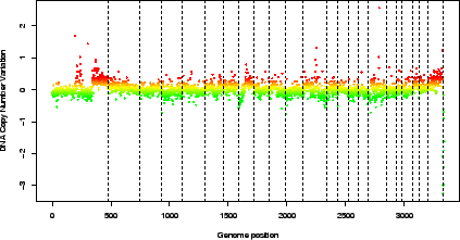
> report.plot(edge.norm, chrLim = "LimitChr", zlim = c(-1, 1)) 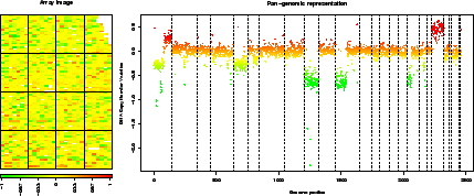 |
> profileCGH <- as.profileCGH(edge.norm$cloneValues)
> profileCGH <- daglad(profileCGH, smoothfunc = "lawsglad", lkern = "Exponential",
+     model = "Gaussian", qlambda = 0.999, bandwidth = 10, base = FALSE,
+     round = 2, lambdabreak = 6, lambdaclusterGen = 20, param = c(d = 6),
+     alpha = 0.001, msize = 5, method = "centroid", nmin = 1,
+     nmax = 8, amplicon = 1, deletion = -5, deltaN = 0.1, forceGL = c(-0.15,
+         0.15), nbsigma = 3, MinBkpWeight = 0.35, verbose = FALSE)
[1] "Smoothing for each Chromosome"
[1] "Optimization of the Breakpoints"
[1] "Check Breakpoints Position"
> edge.norm$cloneValues <- as.data.frame(profileCGH)
> edge.norm$cloneValues$ZoneGNL <- as.factor(edge.norm$cloneValues$ZoneGNL)
> data(qscores)
> qscore.list <- list(smoothness = smoothness.qscore, var.replicate = var.replicate.qscore,
+     dynamics = dynamics.qscore)
> edge.norm$quality <- qscore.summary.arrayCGH(edge.norm, qscore.list)
> edge.norm$quality
              name                                     label score
1 LOCAL_SMOOTHNESS Local signal variability along the genome 0.021
2    VAR_REPLICATE      Average variability among replicates 0.011
3  SIGNAL_DYNAMICS Dynamics of the DNA copy number variation 0.399
Function html.report generates an HTML file with key features of the normalization process: array image and genomic profile before and after normalization, spot-level flag report, and value of the quality criteria.
> html.report(edge.norm, dir.out = ".", array.name = "an array with local bias",
+     chrLim = "LimitChr", light = FALSE, pch = 20, zlim = c(-2,
+         2), file.name = "edge")
The results of the previous command can be viewed in the file edge.html.
> spot.names <- c("Clone", "FLAG", "TEST_B_MEAN", "REF_B_MEAN",
+     "TEST_F_MEAN", "REF_F_MEAN", "ChromosomeArm")
> clone.names <- c("Clone", "Chromosome", "Position", "Validation")
> ac <- import(paste(dir.in, "/gradient.gpr", sep = ""), type = "gpr",
+     spot.names = spot.names, clone.names = clone.names, sep = "\t",
+     comment.char = "@", add.lines = TRUE)
[1] "number of lines does not match array design: adding empty lines..."
[1] "calculating array design..."
> ac$arrayValues$F1 <- log(ac$arrayValues[["TEST_F_MEAN"]], 2)
> ac$arrayValues$F2 <- log(ac$arrayValues[["REF_F_MEAN"]], 2)
> ac$arrayValues$B1 <- log(ac$arrayValues[["TEST_B_MEAN"]], 2)
> ac$arrayValues$B2 <- log(ac$arrayValues[["REF_B_MEAN"]], 2)
> Ratio <- (ac$arrayValues[["TEST_F_MEAN"]] - ac$arrayValues[["TEST_B_MEAN"]])/(ac$arrayValues[["REF_F_MEAN"]] -
+     ac$arrayValues[["REF_B_MEAN"]])
> Ratio[(Ratio <= 0) | (abs(Ratio) == Inf)] <- NA
> ac$arrayValues$LogRatio <- log(Ratio, 2)
> gradient <- ac
> data(spatial)
> data(flags)
> flag.list <- list(local.spatial = local.spatial.flag, spot = spot.flag,
+     SNR = SNR.flag, global.spatial = global.spatial.flag, val.mark = val.mark.flag,
+     position = position.flag, unique = unique.flag, amplicon = amplicon.flag,
+     chromosome = chromosome.flag, replicate = replicate.flag)
> gradient.norm <- norm.arrayCGH(gradient, flag.list = flag.list,
+     FUN = median, na.rm = TRUE)
[1] "local.spatial"
[1] "mean of unbiased zone :  8.39530436452067"
[1] "There is no spatial bias"
  zone.number       mu effectif effectif.cumul frequency.cumul biased.zone
1           7 8.693635      510            510      0.05083732           0
2           6 8.606773      626           1136      0.11323764           0
3           5 8.494905     1083           2219      0.22119219           0
4           4 8.469920     2510           4729      0.47139155           0
5           3 8.409388     2520           7249      0.72258772           0
6           2 8.349206     2222           9471      0.94407895           0
7           1 8.180788      561          10032      1.00000000           0
[1] "spot"
[1] "SNR"
[1] "global.spatial"
[1] "val.mark"
[1] "position"
[1] "unique"
[1] "amplicon"
[1] "chromosome"
[1] "replicate"
> gradient.norm <- sort.arrayCGH(gradient.norm)
> profileCGH <- as.profileCGH(gradient.norm$cloneValues)
> profileCGH <- daglad(profileCGH, smoothfunc = "lawsglad", lkern = "Exponential",
+     model = "Gaussian", qlambda = 0.999, bandwidth = 10, base = FALSE,
+     round = 2, lambdabreak = 6, lambdaclusterGen = 20, param = c(d = 6),
+     alpha = 0.001, msize = 5, method = "centroid", nmin = 1,
+     nmax = 8, amplicon = 1, deletion = -5, deltaN = 0.1, forceGL = c(-0.15,
+         0.15), nbsigma = 3, MinBkpWeight = 0.35, verbose = FALSE)
[1] "Smoothing for each Chromosome"
[1] "Optimization of the Breakpoints"
[1] "Check Breakpoints Position"
> gradient.norm$cloneValues <- as.data.frame(profileCGH)
> gradient.norm$cloneValues$ZoneGNL <- as.factor(gradient.norm$cloneValues$ZoneGNL)
> data(qscores)
> qscore.list <- list(smoothness = smoothness.qscore, var.replicate = var.replicate.qscore,
+     dynamics = dynamics.qscore)
> gradient.norm$quality <- qscore.summary.arrayCGH(gradient.norm,
+     qscore.list)
> gradient.norm$quality
              name                                     label score
1 LOCAL_SMOOTHNESS Local signal variability along the genome 0.032
2    VAR_REPLICATE      Average variability among replicates 0.050
3  SIGNAL_DYNAMICS Dynamics of the DNA copy number variation 0.294
Function html.report generates an HTML file with key features of the normalization process: array image and genomic profile before and after normalization, spot-level flag report, and value of the quality criteria.
> html.report(gradient.norm, dir.out = ".", array.name = "an array with spatial gradient",
+     chrLim = "LimitChr", light = FALSE, pch = 20, zlim = c(-2,
+         2), file.name = "gradient")
The results of the previous command can be viewed in the file gradient.html.